Finding the Local Optimal Number of Hidden Nodes in a Neural Network
By Priscilla Jenq (pjj)
Final Writeup
Summary
I implemented, from scratch, a sequential version of an Artificial Neural Network (ANN) that trains and tests stock data with varying number of hidden nodes. My parallel implementation used OpenMP to optimize for performance on a CPU. Analysis of the program's performance was done on the GHC machines using various number of threads.
Background
Artificial Neural Networks (ANNs) are very popular and powerful technique used in
machine learning. ANNs are composed of a “number of highly interconnected processing
elements” [Stergiou] working in parallel to solve specific problems. They are used
to extract patterns and find trends from large sets of data that humans or computers may not be
able to detect. These neural networks are usually organized into layers that are comprised of a
number of nodes that are connected to each other. The three main types of layers are the input layer,
hidden layer(s), and output layer. ANNs usually contains rules for learning that “modifies
weights of the connections according to the input patterns that it is presented with” [ref], and
these patterns are shown to the network by way of the input layer. There may be one or more
hidden layers and these layers do the actual processing of data, while the output layer
outputs the answer. Feed forward is a method by which the data is passed through the ANN, going from the input layer, through the hidden layer, to the output layer. The output value will be compared with the actual value to generate an output error. This error will propagate back through the neurons using the gradient descent method, which will calculate the changes in these weight (I refer to these as delta w's). Then, all the weights will be updated by adding delta w's to the old weights, which gives us the new weights. The purpose of updating the weights is to reduce the output error. After training all the input data in one iteration, hopefully one can reduce the total error in terms of the MSE (which is defined below).
For this project, I studied the application of ANNs in the financial industry by building and analyzing an ANN to do stock market predictions. The goal was to find the local minimum number of hidden nodes in a single hidden layer that would be able to achieve the best prediction in terms of accuracy. I chose to work with one hidden layer because while researching NNs, I found that adding more and more layers would become computationally expensive pretty quickly while only a relatively small amount of improvements in performance would be seen.
This problem can benefit greatly from parallelism because most people usually try to find the number of hidden nodes to use through either trial and error or simply by just using the same number of nodes in input layer, both of which can be very ineffective. With parallelism, I was able to speed up the process of finding a local optimal number of hidden nodes for fairly accurate stock price predictions.
The key data structure for this project is given in ann.h, which defines the ANN data structure. It consists of fields that hold information about the ANN, such as the number of input nodes, hidden nodes and output nodes, and also contains fields that are meant for training the system. Examples of the latter include matricies (2D arrays) that hold weight and changes in weight (aka the "delta w's"), as well as vectors that hold the links (pointers) in and out of the nodes in each layer, and arrays that store the error, which is used in backward propagation, when updating the weights.
Data, given in data.h, is the other key data structure and its purpose is for holding the training data. When the program reads in the input CSV file, which consists of 6 columns (attributes), it stores the number of rows and number of columns, the filename, and also contains two 2D arrays, which holds the input data and the normalized data.
The input to the ANN is a CSV file with 6 attributes and the output is the predicted next day's open price for the stock. Something to note is that for this project, I worked data that was downloaded from the Yahoo finance site. I mainly chose to work with 3 years worth of data, that is, stock data over a period of three years from the current day. The spreadsheet downloaded contains 7 columns: date, open price, close price, high, low, adjusted close and volume. The data is also given as most recent day first and one day is represented by one row. (So for three years, this is about 252*3 = 756 rows). So I had to preprocess the data first (take out the date column and re-order the rows so that the most recent day's data is the last row rather than the first row) before exporting as a CSV that could be given as input to the ANN. I got three year data from different companies in different sectors (financial, utilities, high tech...etc) and the input I worked with include BOA (Bank of America), T (AT&T), XOM (Exxon Mobile) and GOOG (Google).
As a side note, some of the terminology that I will use are explained below:
MSE (mean squared error): This value is one of the criteria to stop the training of the neural network. MSE is defined as the sum of the square of errors of outputs divided by the total number of cases involved in the training. The error used here is defined as the difference between the actual (target) value and the predicted value generated from the ANN. (Note that there are other methods to compute the MSE, such as using validation data set to stop the training by checking if total number of accuracy is improved and if total accuracy hasn’t, then one can stop the training. I did not use this method to stop the training in this project. To stop training, I set a tolerable error and a maximum cycle, and the one that was reached first would stop the training.)
Accuracy: Because the predicted price and the actual price must change in the same direction to be considered a good prediction for the stock market (and can at least help us to make the decision to either buy, sell or hold), accuracy can be defined as the number of same directional changes of predictions divided by total number of testing cases. I called this the "hit ratio." Another way to define it is to say that a lower MSE means a higher accuracy because it shows how close the predicted value is from the target value for the values that change in the same direction.
Approach
Technologies
I used C/C++ in this project and used OpenMP in order to parallelize my implementation. I also used the GHC machines to run my program and test for performance. The GHC machines consist of 8 cores and 2 execution contexts per core, which means 16 execution contexts.
Algorithm
The pseudo code of my program is outlined below.
- Process command line arguments and set corresponding variables of the program
- Read in data file and put the data cases into data array for future reference.
- Process the data by normalization so the data values will be converted from arbitrary values to values between -1 and +1
- Initialize ANNs // the number of ANNs to be trained and tested
- Parallel do the following using ANN with different hidden layer configuration {
- While (MSE > tolerable error && cycle < maximum cycle) {
- For all training data do {
- Forward-propagation
- Backward propagation of errors
- Update weights
- }
- Compute MSE
- }
- // test this ANN
- Test run current ANN with test data
- Compute accuracy
- }
My first approach was to parallelize the execution of training of all configured ANNs to run concurrently (line 6). This means that each n node ANN would be assigned to a specific thread run. This approach allowed me to learn the workload of each segment of the program code during different iterations of the program. It was obvious that assigning a different number of hidden nodes to an ANN required different efforts, i.e., for an ANN with small hidden layer nodes, one can accomplish the training and testing quicker than the ANN with higher number of hidden nodes. Since I assigned a dedicated thread to work on an ANN, this approach gave the situation of an unbalanced workload among various threads (since a thread working on an ANN with 1 hidden node, for example, will obviously finish faster than a thread working on an ANN with 9 hidden nodes). So even though there was some speedup with static scheduling, I felt that this could be improved.
In order to parallelize even further, I considered line 7, which trains the network by going through one data item at a time. Each time, it goes through the forward phase, backward phase and then modifies the weights after finding the gradients using the gradient descent method. This is the so-called stochastic method (also known as online method or incremental method in various internet literatures). So instead of updating the weights one at a time, the weights can be modified as a collection, i.e., compute the weight changes (the gradients of weight change based on the error that was back propagated from the output layer) of all data items and keep these weight changes in a temporary data structure. After processing all data items, the weights can be updated in parallel by adding up all the weight changes for each item all together. This method is usually known as batch method.
The next iteration of my implementation attempted to use the batch method to update all the weights in parallel. I thought that this would significantly improve the run time, but I found that even though this version was running the same program as my first parallel version, it did not give the expected results and actually took a little longer to run than my first version. I conjecture that the reason this method took a longer time is because of overhead due to synchronization. For example, the hit variable needed to be synchronized (since it's being updated) and since I also tried to change delta w inside the loop, I also needed to sync those variables. So from what I observed from these results, I decided to go back to my previous parallel implementation.
My previous parallel implementation used static scheduling, which resulted in the problem of the imbalanced workload, as mentioned before. To resolve this, I changed to dynamic scheduling instead and experimented with an increasing counter in the for loop (ie: iterating from 0 to total_ann) and a decreasing counter in the for loop (iterating from total_ann to 0) to see if they would affect total time spent. The reason why I tested the program's performance with incrementing and decrementing the for loop counter, as well as the results I got from my tests, are explained further in the results section below.
Results
The input to the ANN is a CSV file containing stock data over a certain period of time. I chose to mainly work with three year data, with the exception of the stock data that I used for Yahoo, which covered a span of 10 years. The input data is inter-day and has six attributes: open price, close price, high, low, adjusted close price and volume.
I used the CycleTimer module from past assignments to evaluate performance of my implementation by measuring the time it took to train the data, test the data and the total time.
I was able to run a lot of different input files with varying parameters (ie: training set size, testing set size, schedule type, number of max hidden nodes to consider,...etc.), but for the sake of keeping this section (relatively) short, I limited the graphs shown to data from just a subset of the outputs I got.
In the following paragraphs, I will first evaluate the implications of the results with regards to the goal posed for this project, and then I will analyze the results in terms of themes relevant to what we've learned in 418.
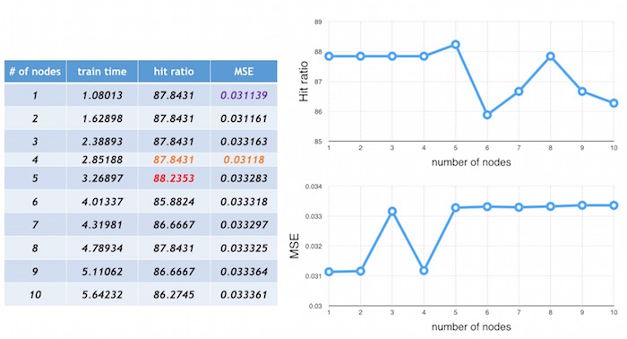
accuracy: I defined accuracy with consideration to the the MSE and hit ratio (explained above in the background section). Below is a snapshot from running Yahoo's 10 year stock data on the ANN with four threads. These results show that the practice of choosing the number of hidden nodes to be equal to number of input layer nodes is not necessarily the best course of action (and I found this to be consistent over all the results I got from running other stock data). In the chart below, notice that that having 5 hidden nodes in an ANN resulted in the best hit ratio (in red) and having 1 hidden node in the ANN gave the 2nd best hit ratio (and having 2, 3, and 4 hidden nodes gave the same hit ratio). Also note that an ANN with 4 hidden nodes resulted in the second best hit ratio and the best mean squared error (in orange). So having 6 hidden nodes, which people might usually choose to use, actually didn't have a better hit ratio or accuracy.
What I learned from doing this project is that it's actually not that easy to find the "best" number of hidden nodes for accuracy that will be true for all stocks, simply because every company is different. For example, blue chip companies are stable, so their stock prices do not fluctuate as much, while other companies that are high risk are more volatile, so their stock prices will vary greatly. There are a lot of other factors that also affect stock prices, like time of year, holidays, world events, weather,...etc that need to be taken into consideration. Depending on all these different factors, the optimal number of hidden nodes will vary from company to company. What I can conclude is that the local optimum number of hidden nodes is not necessarily the number of input layer nodes, as shown in above.
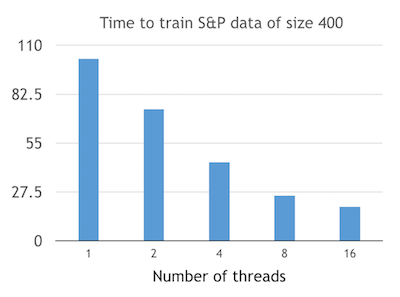
So why is parallelism needed? The graph below shows that using more threads to run the data will result in a lesser amount of time spent on training the data. Here, I used a data set of size 400 from the S&P 500 index. The data set is trained using tolerable error of 0.005 and the maximum cycle is set to 10000, while the learning rate is 0.01. The number of threads shown on the following diagram are 1, 2, 4, 8, and 16.
static vs dynamic scheduling: One of the things we learned in 418 is that static scheduling is better if the workload of tasks to be parallelized are more or less the same. On the other hand, dynamic scheduling will be optimal when the workloads are different. I realized that since the workload is monotonically increasing (ie: a lower number of hidden nodes means there will be less work being done), then a larger number of nodes in the ANN will result in more work being done, which thus means a longer amount of time to execute the task. But if we know which tasks will take the longest beforehand, then threads should be assigned to do those tasks first.
The three graphs below show the differences between the implementation with static scheduling, dynamic scheduling with the smallest number of hidden nodes first, and dynamic scheduling with the largest number of hidden nodes first. The charts on the left detail the order of the nodes run and the thread that each node was assigned to, and the graphs on the right shows for each thread, the amount of time it took to run the n hidden node ANN that was assigned to it. I ran the ANN using Yahoo's stock data over a period of 10 years as input, with a train size of 300 and test size of 256, and four threads.
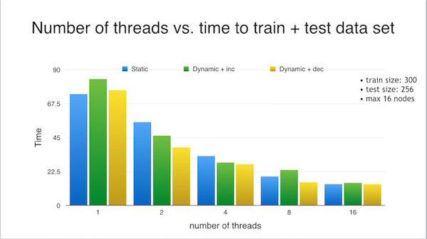
I found from my results that the "largest first" dynamic scheduling gave the fastest results in terms of time taken to train the data. Below, I show the differences in training time depending on the different schedules, for various number of threads. Note that in the graph below (and elsewhere), "dynamic + dec" refers to the "largest first" dynamic scheduling (since the counter is being decremented) and "dynamic + inc" refers to "smallest first" dynamic scheduling since the counter was being incremented.
The ANN was trained with a data set of size 300, tested with 256 units of data and tried every ANN configuration from 1 to 16 hidden nodes. Notice that for 1 thread, static scheduling actually better than dynamic scheduling. This makes sense because there is overhead to dynamic scheduling. After each iteration, the threads have to stop and get a new value of the loop variable to use for its next iteration. But in the case of one thread, that thread is doing all the work anyway, so "stopping and getting" the new value is unneccessary time spent.
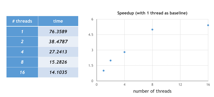
Speedup is defined as the execution time of using only one thread divided by the execution time when multiple threads are used. The graph below illustrates the speedup achieved when running the program with "largest first" dynamic scheduling for an ANN of n hidden nodes (for n = 1 to 10) and using a training set of size 300 and test size 256. The execution of the program on one thread was used as a baseline, and a 5.4 x speedup was achieved when using 16 threads. Notice that after a certain number of threads, the speedup--while it still exists--is not as drastic as before. I imagine that this is probably because there's overhead associated with creating threads and if the range of hidden nodes we're running the ANNs with isn't super large, then there's less of a benefit from using so many threads.
In the graph below, I attempted to map out the training time vs the testing time when running the 10 year stock data with training set size 300 and testing set size 256 with dynamic scheduling (largest node first). However, the times for testing were so small that they didn't show up visibly on the graph :(. So I included a chart of the training time and testing time with regards to each n hidden node ANN, for n from 1 to 10. For reference, this is a link to the spreadsheet version of my results. It gives the time spent on training, testing, the number of "hits" and the hit ratio, as well as the total time it took to run for each ANN configuration of n hidden nodes, and for various number of threads. The two approaches to scheduling I took note of and showed in the doc was static scheduling and dynamic scheduling + largest node first.
Possible future work
- Expand the data set to include other sectors and companies, not just the ones used in this project
- Now that we can figure out the minimum and best number of hidden nodes for first hidden layer, can we expand to compute the next hidden layer if we want to have deep learning? If the answer is yes, can we fix the first hidden layer architecture (i.e., fix its number of hidden nodes that we found) and then continue to find the optimal hidden node number for second hidden layer? This approach would be similar to the greedy method of algorithm development. The question is: will this approach really will give us the optimal numbers?
- The choosing of initial weights of neural network determine if one can fast approach to global minimum or will be stocked in local minimum. Can we somehow use parallel processing technique to find the best starting points for all these weights? Brute force may not be a good idea since the complexity is too high. But how about the greedy method mentioned above if we can fix the weight of a link and incrementally fix other weights from there?
- Today's web services have become popular, so can we somehow use the request/response approach to find the best neural network in our stock prediction application (or in any applications)?
References
- To familiarize myself with Artificial Neural Networks, I watched a multi-part series of videos introducing them. I also read through a paper from Imperial College London introducing ANNs and a page from UWisconsin discussing the basics. This post was also helpful in understanding some questions regarding the different layers and typical number of hidden nodes used.
- 15-418 Lecture 24 slides regarding backpropagation and gradient descent were also helpful
Thanks!
Thanks to Prof. Kayvon and Prof. Bryant for a challenging and thought-provoking semester! I learned a lot and I know that this knowledge will be invaluable, especially once I start working full-time after graduation. (YAY!)